Multitasking: Good for computers, bad for people.

See if you can read this to the end without answering the phone, noticing a notification, etcetera:

https://fee.org/articles/multitasking-is-bad-for-your-brain/?utm_source=FEE+Email+Subscriber+List&utm_campaign=46f69810ec-MC_FEE_WEEKLY_2017_06_30&utm_medium=email&utm_term=0_84cc8d089b-46f69810ec-108080753

Matrix inversion, row ops, program added

The row operation matrix inversion method is so neat and ingenious, and it has the same operations for all dimensions of matrix.

Here is a step by step approach, where firstly the dimension is chosen, then the first of the buttons is selected (Start). After which the buttons are selected in order. The states of the left and right matrices are displayed at each stage, and finally the identity matrix appears on the left, and the inverse of the original matrix appears on the right.

http://mathcomesalive.com/mathsite/matrix%20prog%203.html

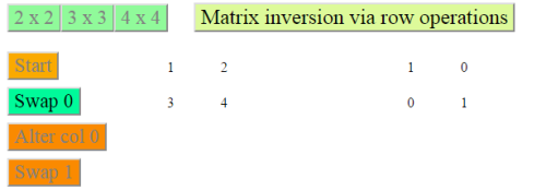
The first display shows the original matrix on the left. Nothing has been done yet.

 

The second one is the 2 x 2 matrix inverted.

The third is the 4 x 4 matrix inverted.

The matrices can be altered with the file name for the application, “matrix prog 3.html”. using right click and “view page source”. You are then on your own, with javascript !!!!!!!!

Matrix inversion made relatively easy

This is the standard way of inverting a matrix. I came across this first in 1960. Oh so long ago! Goodbye Cramer’s Rule.

Part 4: Tuning the feedback controller

Our first order process is described by the equation y_n+1 = ay_n + kx_n , where y_n is the process output now (at time n),  x_n is the process input between time n and time n+1, and y_n+1 is the process output at time n+1.
a is the coefficient determining how quickly the process settles after a change in the input, and k is related to the process steady state gain (ratio of settled output to constant input).

If we set the input to be a constant x and the output settled value to be a constant y, then

y = ay + kx, and solving for y/x we get y/x = k/(1-a), the actual steady state gain.

In what follows the k will represent the actual steady state gain, the old k divided by (1-a)

The fist two plots show the process alone, with input set to 6 at time zero. In the first the steady state gain is set to 1, and in the second it is set to 2

Now we look a t the process under “direct” control, where the input is determined only by the chosen setpoint value. The two equations are

y_n+1 = ay_n + kx_n  and  x_n = Ad_n  (direct control: h is zero)

To obtain a controlled system with overall steady state gain equal to 1 (settled output  equal to desired output) it is easy to see that  A has to be equal to (1-a)/k

It is not so obvious how the choice of h affects the performance of the controlled system. To do this we observe that the complete system is described entirely by the process equation and the controller equation together, and we can eliminate the x_n from the two equations to get y_n+1 = ay_n + k(Ad_n + h(y_n – d_n))

which rearranged is y_n+1 = (a + kh)y_n + k(A – h)d_n 

Substituting   (1-a)/k for A, as found above, gives  y_n+1 = (a + kh)y_n + (1 – a – kh)d_n 

which has the required steady state gain of 1.

This final equation has the SAME structure as the process equation,
with a + kh in place of a

So now we will see how the value of the “a” coefficient affects the dynamic response of the system.

If h > 0 the controlled system will respond slower than with h = 0, and if h < 0 it will respond faster:

Setpoint changes were made at time 20 and at time 40

Congratulations if you got this far. This introduction to computer controlled processes has been kept as simple as possible, while using just the minimum amount of really basic math. The difficulties are in the interpretation and meaning of the various equations, and this something which is studiously avoided in school math. Such a shame.

Now you can run the program yourself, and play with the coefficients. It is a webpage with javascript:  http://mathcomesalive.com/mathsite/firstordersiml.html

Aspects and theoretical stuff which follow this (not here !) include the  backward shift operator z and its use in forming the transfer function of the system, behaviour of systems with wave form inputs to assess frequency response, representation of systems in matrix form (state space), non-linear systems and limit cycles, optimal control, adaptive control, and more…..

Part 3: Computer control of real dynamic systems

Let us return to the industrial steam engine driving a range of equipment, each piece in the charge of an operator. In order to keep the factory working properly it is necessary to keep the speed of the steam engine reasonably constant, at what is called the desired output, or the set point. A human controller can achieve this fairly well, by direct observation of the speed and experience of the effect of changing the steam flow rate, but automatically? Well, James Watt solved the problem with a mechanical device (details later). We will now see how to “do it with a computer”.

Diagram of the physical system. There will be a valve on the steam line (not shown).

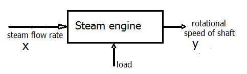
The information flow diagram. The load is not measured, and may vary.

Now we have a controller in the picture, fed with two pieces of information, the current speed and the desired speed. The controller can be human, mechanical or computer based. It has a set of rules to figure out the appropriate steam flow rate.

Now we have computer control. The output of the system is measured (sampled) at regular intervals, the computer calculates the required flow rate , sends the corresponding value to the valve actuating mechanism, which holds this value until the next sampling time, when the process is repeated. Using n=1, 2, 3, ….. for the times at which the output is sampled and the controller does its bit, we have at time n the speed measure y_n, the desired speed d_n and the difference between them (or error in the speed), and they are used to calculate the system input x_n with the formula shown in the controller box.

The equation in the steam engine box is our fairly simple first order linear system model as described in the previous post. It is a good idea to have a model of the process dynamics for many reasons (!), one of which is that we can do experiments on the whole controlled system by simulation rather than on the real thing.

Looking at the controller function (formula), x_n = Ad_n + h(y_n – d_n) , it is “obvious” that if the coefficient h is zero we have direct control (no feedback), and so the value of the coefficient A must be chosen accordingly (see next post).

It is not so obvious how the choice of h affects the performance of the controlled system. To do this we observe that the complete system is described entirely by the process equation and the controller equation together, and we can eliminate the x_n from the two equations to get y_n+1 = ay_n + k(Ad_n + h(y_n – d_n))

which rearranged is y_n+1 = (a + h)y_n + k(A – h)d_n 

and has the SAME structure as the process equation, with a + h in place of a

In the next post, on tuning our controller, we will see how the value of the “a” coefficient affects the dynamic response of the system.

Time Series and Discrete Processes, or Calculus Takes a Back Seat

 

In the business and manufacturing world data keeps on coming in. What is it telling me? What is it telling me about the past? Can it tell me something believable about the future. These streams of data form the food for “time series analysis”, procedures for condensing
the data into manageable amounts.

Here is a plot of quarterly Apple I-phone sales. (ignore the obvious error, this is common)

I see several things, one is a pronounced and fairly regular variation according to the quarter, another is an apparent tendency for the sales to be increasing over time, and the third is what I will call the jiggling up and down, more formally called the unpredictable or random behaviour.
The quarterly variation can be removed from the data by “seasonal analysis”, a standard method which I am not going to deal wirh (look it up. Here’s a link:

https://onlinecourses.science.psu.edu/stat510/node/69
The gradual increase, if real, can be found by fitting a straight line to the data using linear regression, and then subtracting the line value from the observed value for each data point. This gives the “residuals”, which are the unpredictable bits.

Some time series have no pattern, and can be viewed as entirely residuals.
We cannot presume that the residuals are just “random”, so we need a process of smoothing the data to a) reveal any short term drifting, and b) some help with prediction.
The simple way is that of “moving average”, the average of the last k residuals. Let’s take k = 5, why not !
Then symbolically, with the most recent five data items now as x(n), x(n-1),..,x(n-4), the moving average is

ma = (x(n)+x(n-1)+x(n-2)+x(n-3)+x(n-4))/5

If we write it as ma = x(n)/5 + x(n-1)/5 + x(n-2)/5 + x(n-3)/5 + x(n-4)/5 we can see that this is a weighted sum of the last five items, each with a weight of 1/5 (the weights add up to 1).
This is fine for smoothing the data, but not very good for finding out anything about future short term behaviour.
It was figured out around 60 years ago that if the weights got smaller as the data points became further back in time then things might be better.

Consider taking the first weight, that applied to x(n) as 1/5, or 0.2 so the next one back is 0.2 squared and so on. These won’t add up to 1 which is needed for an average, so we fix it.
0.2 + 0.2^2 + 0.2^3 + … is equal to 0.2/(1-0.2) or 0.2/0.8 so the initial weights all need to be divided by the 0.8, and we get the “exponentially weighted moving average” ewma.

ewma(n) =
x(n)*0.8+x(n-1)*0.8*0.2+x(n-2)*0.8*0.04+x(n-3)*0.8*0.008+x(n-)*0.8*0.0016 + …… where n is the time variable, in the form 1, 2, 3, 4, …

A quick look at this shows that ewma(n-1) is buried in the right hand side, and we can see that ewma(n) = 0.2*ewma(n-1) + 0.8*x(n),
which makes the progressive calculations very simple.
In words, the next value of the ewma is a weighted average of the previous value of the ewma and the new data value. (0.2 + 0.8 = 1)

The weighting we have just worked out is not very useful, as it pays too much attention to the new data, and the ewma will therefore be almost as jumpy as the data. Better values are in the range 0.2 to 0.05 as you can see in the following pictures, in which the k value is the weighting of the data value x, and the weighting of the ewma value is then (1-k):

So the general form is ewma(n) = (1-k)*ewma(n-1) + k*x(n)

With k=0.5 we do not get a very good idea of the general level of the sequence, as the ewma value is halfway between the data and the previous ewma value, so we try k=0.1

Much better, in spite of my having increased the random range from 4 to 10.

Going back to random=4, but giving the data an upward drift the ewma picks up the direction of the drift, but fails to provide a good estimate of current data value. This can be fixed by modifying the ewma formula. A similar situation arises when the data values rise at first and then start to fall (second picture)

Common sense says that to reduce the tracking error for a drifting sequence it is enough to increase the value of k. But that does not get rid of the error. We need a measure of error which gets bigger and bigger as long as the error persists. Well, one thing certainly gets bigger is the total error, so let us use it and see what happens.

Writing the error at time n as err(n), and the sum of errors to date as totalerr(n) we have

err(n) = x(n) – ewma(n), and totalerr(n) = totalerr(n-1) + err(n)

Then we can incorporate the accumulated error into the ewma formula by adding a small multiple of totalerr(n) to get

ewma(n) =  ewma(n) = (1-k)*ewma(n-1) + k*x(n) + h*totalerr(n)

In the first example below h = 0.05, and in the second h = 0.03, as things were too lively with h=0.05.

A good article on moving averages is:
http://www.mcoscillator.com/learning_center/kb/market_history_and_background/who_first_came_up_with_moving_averages/

In my next post I will show how the exponentially weighted moving average can be described in the language of discrete time feedback systems models, as used in modern control systems, and with luck I will get as far as the z-transfer function idea.

CBE and computer programming

What hope can there be for Competency Based Education, by computer of course, if commercial programmers continue to come up with this sort of stuff?