In the business and manufacturing world data keeps on coming in. What is it telling me? What is it telling me about the past? Can it tell me something believable about the future. These streams of data form the food for “time series analysis”, procedures for condensing
the data into manageable amounts.
Here is a plot of quarterly Apple I-phone sales. (ignore the obvious error, this is common)

I see several things, one is a pronounced and fairly regular variation according to the quarter, another is an apparent tendency for the sales to be increasing over time, and the third is what I will call the jiggling up and down, more formally called the unpredictable or random behaviour.
The quarterly variation can be removed from the data by “seasonal analysis”, a standard method which I am not going to deal wirh (look it up. Here’s a link:
https://onlinecourses.science.psu.edu/stat510/node/69
The gradual increase, if real, can be found by fitting a straight line to the data using linear regression, and then subtracting the line value from the observed value for each data point. This gives the “residuals”, which are the unpredictable bits.
Some time series have no pattern, and can be viewed as entirely residuals.
We cannot presume that the residuals are just “random”, so we need a process of smoothing the data to a) reveal any short term drifting, and b) some help with prediction.
The simple way is that of “moving average”, the average of the last k residuals. Let’s take k = 5, why not !
Then symbolically, with the most recent five data items now as x(n), x(n-1),..,x(n-4), the moving average is
ma = (x(n)+x(n-1)+x(n-2)+x(n-3)+x(n-4))/5
If we write it as ma = x(n)/5 + x(n-1)/5 + x(n-2)/5 + x(n-3)/5 + x(n-4)/5 we can see that this is a weighted sum of the last five items, each with a weight of 1/5 (the weights add up to 1).
This is fine for smoothing the data, but not very good for finding out anything about future short term behaviour.
It was figured out around 60 years ago that if the weights got smaller as the data points became further back in time then things might be better.
Consider taking the first weight, that applied to x(n) as 1/5, or 0.2 so the next one back is 0.2 squared and so on. These won’t add up to 1 which is needed for an average, so we fix it.
0.2 + 0.2^2 + 0.2^3 + … is equal to 0.2/(1-0.2) or 0.2/0.8 so the initial weights all need to be divided by the 0.8, and we get the “exponentially weighted moving average” ewma.
ewma(n) =
x(n)*0.8+x(n-1)*0.8*0.2+x(n-2)*0.8*0.04+x(n-3)*0.8*0.008+x(n-)*0.8*0.0016 + …… where n is the time variable, in the form 1, 2, 3, 4, …
A quick look at this shows that ewma(n-1) is buried in the right hand side, and we can see that ewma(n) = 0.2*ewma(n-1) + 0.8*x(n),
which makes the progressive calculations very simple.
In words, the next value of the ewma is a weighted average of the previous value of the ewma and the new data value. (0.2 + 0.8 = 1)
The weighting we have just worked out is not very useful, as it pays too much attention to the new data, and the ewma will therefore be almost as jumpy as the data. Better values are in the range 0.2 to 0.05 as you can see in the following pictures, in which the k value is the weighting of the data value x, and the weighting of the ewma value is then (1-k):
So the general form is ewma(n) = (1-k)*ewma(n-1) + k*x(n)

With k=0.5 we do not get a very good idea of the general level of the sequence, as the ewma value is halfway between the data and the previous ewma value, so we try k=0.1

Much better, in spite of my having increased the random range from 4 to 10.
Going back to random=4, but giving the data an upward drift the ewma picks up the direction of the drift, but fails to provide a good estimate of current data value. This can be fixed by modifying the ewma formula. A similar situation arises when the data values rise at first and then start to fall (second picture)


Common sense says that to reduce the tracking error for a drifting sequence it is enough to increase the value of k. But that does not get rid of the error. We need a measure of error which gets bigger and bigger as long as the error persists. Well, one thing certainly gets bigger is the total error, so let us use it and see what happens.
Writing the error at time n as err(n), and the sum of errors to date as totalerr(n) we have
err(n) = x(n) – ewma(n), and totalerr(n) = totalerr(n-1) + err(n)
Then we can incorporate the accumulated error into the ewma formula by adding a small multiple of totalerr(n) to get
ewma(n) = ewma(n) = (1-k)*ewma(n-1) + k*x(n) + h*totalerr(n)
In the first example below h = 0.05, and in the second h = 0.03, as things were too lively with h=0.05.


A good article on moving averages is:
http://www.mcoscillator.com/learning_center/kb/market_history_and_background/who_first_came_up_with_moving_averages/
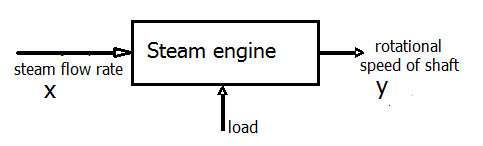
In my next post I will show how the exponentially weighted moving average can be described in the language of discrete time feedback systems models, as used in modern control systems, and with luck I will get as far as the z-transfer function idea.